El teorema del límite central es un teorema fundamental de probabilidad y estadística. El teorema describe la distribución de la media de una muestra aleatoria proveniente de una población con varianza finita. Cuando el tamaño de la muestra es lo suficientemente grande, la distribución de las medias sigue aproximadamente una distribución normal. El teorema se aplica independientemente de la forma de la distribución de la población. Muchos procedimientos estadísticos comunes requieren que los datos sean aproximadamente normales. El teorema de límite central le permite aplicar estos procedimientos útiles a poblaciones que son considerablemente no normales. El tamaño que debe tener la muestra depende de la forma de la distribución original. Si la distribución de la población es simétrica, un tamaño de muestra de 5 podría producir una aproximación adecuada. Si la distribución de la población es considerablemente asimétrica, es necesario un tamaño de muestra más grande. Por ejemplo, la distribución de la media puede ser aproximadamente normal si el tamaño de la muestra es mayor que 50. Las siguientes gráficas muestran ejemplos de cómo la distribución afecta el tamaño de la muestra que se necesita.

Distribución uniforme

Medias de las muestras
Muestras de una población uniforme
Una población que sigue una distribución uniforme es simétrica, pero marcadamente no normal, como lo demuestra el primer histograma. Sin embargo, la distribución de las medias de 1000 muestras de tamaño 5 de esta población es aproximadamente normal debido al teorema del límite central, como lo demuestra el segundo histograma. Este histograma de las medias de las muestras incluye una curva normal superpuesta para ilustrar esta normalidad.

Distribución exponencial

Medias de las muestras
Muestras de una población exponencial
Una población que sigue una distribución exponencial es asimétrica y no normal, como lo demuestra el primer histograma. Sin embargo, la distribución de las medias de 1000 muestras de tamaño 50 de esta población es aproximadamente normal debido al teorema del límite central, como lo demuestra el segundo histograma. Este histograma de las medias de las muestras incluye una curva normal superpuesta para ilustrar esta normalidad.
Python: Central Limit Theorem
The Central Limit Theorem is one of core principles of probability and statistics. So much so, that a good portion of inferential statistical testing is built around it. What the Central Limit Theorem states is that, given a data set – let’s say of 100 elements (See below) if I were to take a random sampling of 10 data points from this sample and take the average (arithmetic mean) of this sample and plot the result on a histogram, given enough samples my histogram would approach what is known as a normal bell curve.
In plain English
- Take a random sample from your data
- Take the average of your sample
- Plot your sample on a histogram
- Repeat 1000 times
- You will have what looks like a normal distribution bell curve when you are done.

For those who don’t know what a normal distribution bell curve looks like, here is an example. I created it using numpy’s normal method

If you don’t believe me, or want to see a more graphical demonstration – here is a link to a simulation that helps a lot of people to grasp this concept: link
Okay, I have bell curve, who cares?
The normal distribution of (Gaussian Distribution – named after the mathematician Carl Gauss) is an amazing statistical tool. This is the powerhouse behind inferential statistics.
The Central Limit Theorem tells me (under certain circumstances), no matter what my population distribution looks like, if I take enough means of sample sets, my sample distribution will approach a normal bell curve.
Once I have a normal bell curve, I now know something very powerful.
Known as the 68,95,99 rule, I know that 68% of my sample is going to be within one standard deviation of the mean. 95% will be within 2 standard deviations and 99.7% within 3.

So let’s apply this to something tangible. Let’s say I took random sampling of heights for adult men in the United States. I may get something like this (warning, this data is completely made up – do not even cite this graph as anything but bad art work)

But reading this graph, I can see that 68% of men are between 65 and 70 inches tall. While less than 0.15% of men are shorter than 55 inches or taller than 80 inches.
Now, there are plenty of resources online if you want to dig deeper into the math. However, if you just want to take my word for it and move forward, this is what you need to take away from this lesson:
p value
As we move into statistical testing like Linear Regression, you will see that we
are focus on a p value. And generally, we want to keep that p value under 0.5. The purple box below shows a p value of 0.5 – with 0.25 on either side of the curve. A finding with a p value that low basically states that there is only a 0.5% chance that the results of whatever test you are running are a result of random chance. In other words, your results are 99% repeatable and your test demonstrates statistical significance.

https://www.youtube.com/watch?v=Ecs_JPe9gCM
| import numpy as np | |
| import random | |
| # Create a parent distribution, from the gamma family | |
| shape, scale = 2., 2. # mean=4, std=2*sqrt(2) | |
| s = np.random.gamma(shape, scale, 100000) | |
| print(np.mean(s)) | |
| import matplotlib.pyplot as plt | |
| import scipy.special as sps | |
| plt.hist(s) | |
| plt.show() | |
| # The distribution of the means from the sampled groups is normally distributed | |
| samples = [ np.mean(random.choices(s, k=20)) for _ in range(1000) ] | |
| plt.hist(samples) | |
| plt.show() |
An illustration of the central limit theorem. The histogram in each panel shows the distribution of the mean value of N random variables drawn from the (0, 1) range (a uniform distribution with  and W = 1; see eq. 3.39). The distribution for N = 2 has a triangular shape and as N increases it becomes increasingly similar to a Gaussian, in agreement with the central limit theorem. The predicted normal distribution with and
  is shown by the line. Already for N = 10, the “observed” distribution is essentially the same as the predicted distribution.
and W = 1; see eq. 3.39). The distribution for N = 2 has a triangular shape and as N increases it becomes increasingly similar to a Gaussian, in agreement with the central limit theorem. The predicted normal distribution with and is shown by the line. Already for N = 10, the “observed” distribution is essentially the same as the predicted distribution.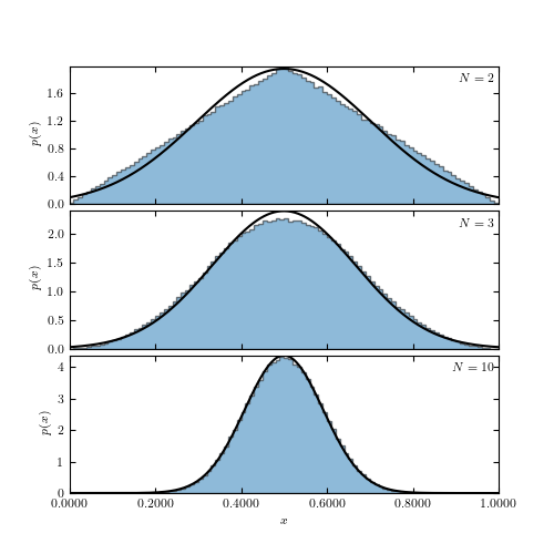

No hay comentarios:
Publicar un comentario